The augmented medallion architecture - Silver Layer
"Silver" layer
Published on : April 15, 2025
| Lastly edited on : April 15, 2025
| 11 minutes read

Lirav DUVSHANI
Series : The augmented medallion architecture
A standard architecture to analytics data platform
"Bronze" layer
"Silver" layer
"Gold" layer
"Platinum" layer
"Parametrization" layer
"Data Quality" layer
The Silver layer - Where the data is cleaned/curated
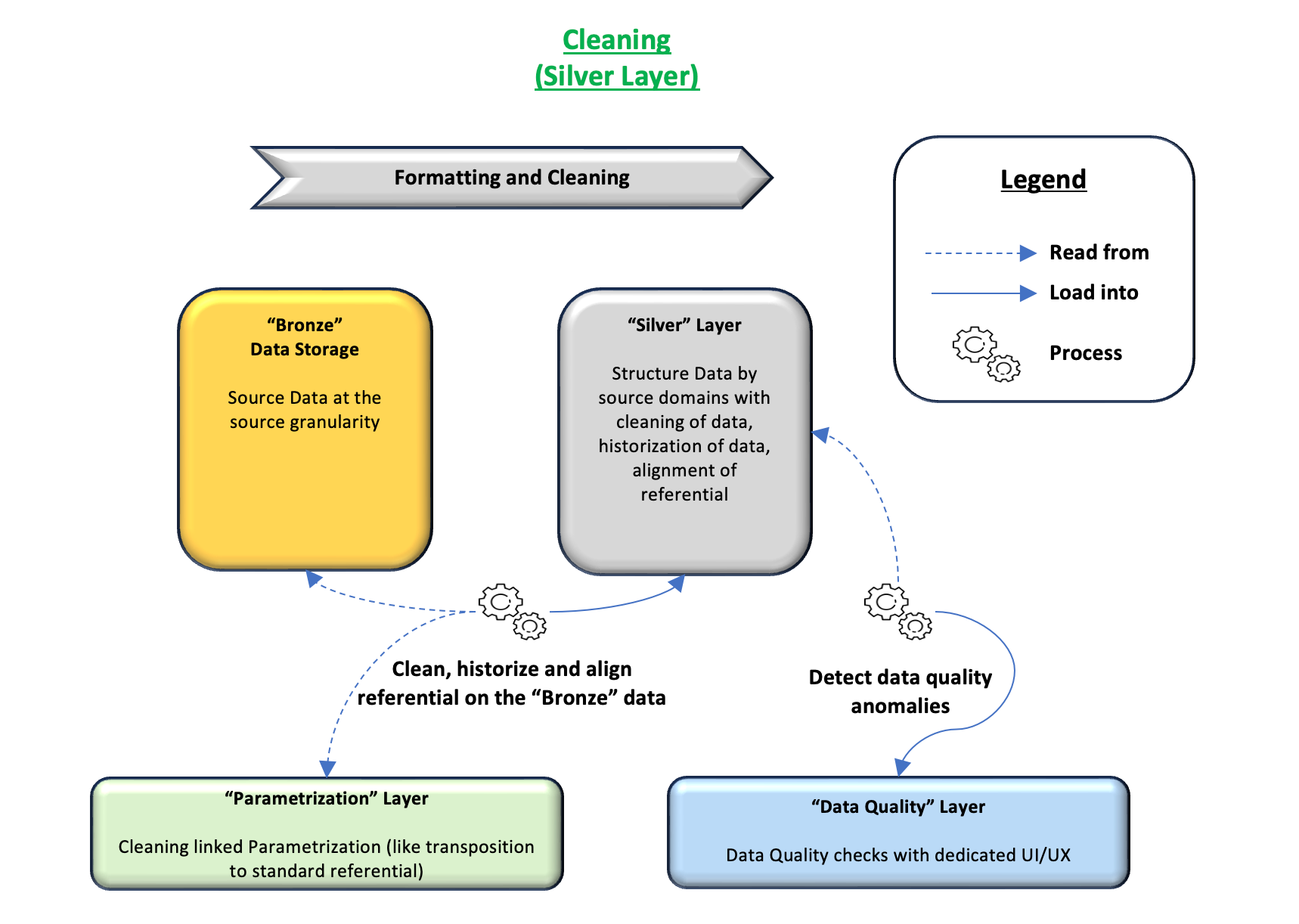
Purpose of the layer
The main purpose of this layer is to provide standardized cleaned and structured data, optimized for analytical use.
The secondary purposes of this layer are to :
- Schema enforcement : Enforce schema to ensure consistency with expected format
- Deduplication & Filtering : Ensure data is accurate and relevant for analytical use
Characteristics of the layer
- Storage should be optimized for analytical use
- The data should be stored in a query-friendly structures, including primary key definition, partitionning and indexing
- Allowed Data Structures
- Structured, can be converted from semi-structured and unstructured data
- Granularity of data
- The data should be detailed, at the same level of granularity as the source data
- Useful metadata information
- All information available in bronze layer
- The extraction timestamp
- The load in bronze layer timestamp (also called ingestion timestamp)
- (if available) The last update of records in the source system
- The load in silver layer timestamp
- All information available in bronze layer
Good practices
In this layer, the transformation applied are mostly cleaning and technical formatting of data (like semi-structured data flattening). For all these transformations, it is very useful to keep inside the Silver layer structure both the original and cleaned data.
This ensures that during data analysis, not only the result of cleaning is available but also the original value prior to cleaning.
As in all the other layers, tracking as much metadata information as possible is very beneficial for data analysis purposes and for monitoring reporting. Among these metadata information, the most important ones would be the source extraction timestamp and the ingestion timestamp.
Standard transformations applied in this layer
- Structure-level Selection and transformation
- Data flattening : Transform semi-structured data in a more user and query friendly format
- Last Available Data selection : Selection of the last version of any record
- Column-level transformations
- Cleaning of the source data
- Technical cleaning : Empty values, which should not be allowed
- Functional cleaning : Incoherent values should be cleaned, like invalid dates or any type of incoherent entries
- Standardization of referentials
- Transposition of source data into custom referential : When multiple sources are present
- Cleaning of the source data
| Transformation Category | Transformation | Use Case | Before Cleaning | After Cleaning |
|---|---|---|---|---|
| Technical Cleaning | Empty values | Fill empty metric values with 0 | NULL 1 | 0 1 |
| Functional Cleaning | Valid Date | Default to NULL if date not coherent | 2024-13-13 2024-02-12 | NULL 2024-02-12 |
| Standardisation of referential | Unify country names into code | Transpose the country names to ISO 3166 alpha-2 | France Fr. Germ. GERMANY | FR FR GE GE |
| Data flattening | Empty values | Fill empty metric values with 0 | {"sector": "Retail", "earnings_range": "<10M"} | Into 2 columns sector = Retail earnings_range = <10M |
Transformation Examples
All the examples are provided considering a storage in a database, e.g. in tables.
Data Flattening
Flattening of a field can be done in multiple way :
- Stored inside a single table
- Stored in multiple tables
Flattening inside a single table
Here is an example of a customer table with a key named "Customer ID".
Bronze Table - Customer
| Customer ID | Customer Name | Customer Tags | Ingestion Timestamp |
|---|---|---|---|
| 1 | Customer A | {"sector": "Industry", "earnings_range": ">100M"} | 2025-01-02T03:55:02.728Z |
| 2 | Customer B | {"sector": "IT", "earnings_range": "10-100M"} | 2025-01-02T03:55:02.728Z |
| 3 | Customer C | {"sector": "Retail", "earnings_range": "<10M"} | 2025-01-02T03:55:02.728Z |
| 1 | Customer A | {"sector": "Industry", "earnings_range": ">100M"} | 2025-01-03T03:52:03.127Z |
| 3 | Customer C | {"sector": "Retail", "earnings_range": "<100M" , "billing_currency": "EUR"} | 2025-01-04T04:02:42.009Z |
Silver Table - Customer
| Customer ID | Customer Name | Sector | Earnings Range | Billing Currency | Ingestion Timestamp | Silver Load Timestamp |
|---|---|---|---|---|---|---|
| 1 | Customer A | Industry | >100M | ∅ | 2025-01-02T03:55:02.728Z | 2025-01-05T05:12:02.000Z |
| 2 | Customer B | IT | 10-100M | ∅ | 2025-01-02T03:55:02.728Z | 2025-01-05T05:12:02.000Z |
| 3 | Customer C | Retail | <10M | ∅ | 2025-01-02T03:55:02.728Z | 2025-01-05T05:12:02.000Z |
| 1 | Customer A | Industry | >100M | ∅ | 2025-01-03T03:52:03.127Z | 2025-01-05T05:12:02.000Z |
| 3 | Customer C | Retail | <100M | EUR | 2025-01-04T04:02:42.009Z | 2025-01-05T05:12:02.000Z |
All the tags have been transformed as columns providing information about a customer.
Flattening in multiple tables
Here is an example of a customer table with a key named "Customer ID".
Bronze Table - Customer
| Customer ID | Customer Name | Customer Tags | Ingestion Timestamp |
|---|---|---|---|
| 1 | Customer A | {"sector": "Industry", "earnings_range": ">100M"} | 2025-01-02T03:55:02.728Z |
| 2 | Customer B | {"sector": "IT", "earnings_range": "10-100M"} | 2025-01-02T03:55:02.728Z |
| 3 | Customer C | {"sector": "Retail", "earnings_range": "<10M"} | 2025-01-02T03:55:02.728Z |
| 1 | Customer A | {"sector": "Industry", "earnings_range": ">100M"} | 2025-01-03T03:52:03.127Z |
| 3 | Customer C | {"sector": "Retail", "earnings_range": "<100M" , "billing_currency": "EUR"} | 2025-01-04T04:02:42.009Z |
Silver Table - Customer (Main)
| Customer ID | Customer Name | Ingestion Timestamp | Silver Load Timestamp |
|---|---|---|---|
| 1 | Customer A | 2025-01-02T03:55:02.728Z | 2025-01-05T05:12:02.000Z |
| 2 | Customer B | 2025-01-02T03:55:02.728Z | 2025-01-05T05:12:02.000Z |
| 3 | Customer C | 2025-01-02T03:55:02.728Z | 2025-01-05T05:12:02.000Z |
| 1 | Customer A | 2025-01-03T03:52:03.127Z | 2025-01-05T05:12:02.000Z |
| 3 | Customer C | 2025-01-04T04:02:42.009Z | 2025-01-05T05:12:02.000Z |
Silver Table - Customer (Tags)
| Customer ID | Sector | Earnings Range | Billing Currency | Ingestion Timestamp | Silver Load Timestamp |
|---|---|---|---|---|---|
| 1 | Industry | >100M | ∅ | 2025-01-02T03:55:02.728Z | 2025-01-05T05:12:02.000Z |
| 2 | IT | 10-100M | ∅ | 2025-01-02T03:55:02.728Z | 2025-01-05T05:12:02.000Z |
| 3 | Retail | <10M | ∅ | 2025-01-02T03:55:02.728Z | 2025-01-05T05:12:02.000Z |
| 1 | Industry | >100M | ∅ | 2025-01-03T03:52:03.127Z | 2025-01-05T05:12:02.000Z |
| 3 | Retail | <100M | EUR | 2025-01-04T04:02:42.009Z | 2025-01-05T05:12:02.000Z |
All the tags have been transformed as columns providing information about a customer.
Last Available Data selection
The last available data selection transformation provides a Silver table which contains only the last available relevant information. Thus, the Silver table could be identical to the table in the source system, with a single record per key.
Here is an example of a product table with a key named "Product ID".
Bronze Table - Customer
| Product ID | Product Name | Product Category | Ingestion Timestamp |
|---|---|---|---|
| 1 | Product A | Wood | 2025-01-02T03:55:02.728Z |
| 2 | Product B | IT Service | 2025-01-02T03:55:02.728Z |
| 3 | Product C | Clothes | 2025-01-02T03:55:02.728Z |
| 1 | Product A | Floors - Wood | 2025-01-03T03:52:03.127Z |
| 3 | Product C | Women's clothes | 2025-01-04T04:02:42.009Z |
Silver Table - Customer
| Product ID | Product Name | Product Category | Ingestion Timestamp | Silver Load Timestamp |
|---|---|---|---|---|
| 2 | Product B | IT Service | 2025-01-02T03:55:02.728Z | 2025-01-05T05:12:02.000Z |
| 1 | Product A | Floors - Wood | 2025-01-03T03:52:03.127Z | 2025-01-05T05:12:02.000Z |
| 3 | Product C | Women's clothes | 2025-01-04T04:02:42.009Z | 2025-01-05T05:12:02.000Z |
Only the last record for "Product ID" 1 and 3, based on the ingestion timestamp, have been selected and loaded into the silver table
Data Cleaning
Whatever the format of the source data in Bronze, in the Silver layer, the data should be clean and ready to used to analysis, reporting and any kind of analysis.
Here is an example of a purchase order table with a key named "Purchase Order ID".
This presents all the steps from Bronze, including the selection of the latest available data.
Bronze Table - Order
| Purchase Order ID | Customer Name | Product Name | Order Status | Order Unit Of Measure | Order Quantity | Billing Currency | Billed Amount | Ingestion Timestamp |
|---|---|---|---|---|---|---|---|---|
| PO-1 | Customer 1 | Product A | Invoiced | PC | 3 | EUR | 10,02 | 2025-01-02T03:55:02.728Z |
| PO-2 | Customer 1 | Product B | Ordered | PC | 1002 | USD | 35,99 | 2025-01-02T03:55:02.728Z |
| PO-3 | Customer 2 | Product C | Planned | ∅ | 30 | GBP | 20,00 | 2025-01-02T03:55:02.728Z |
| PO-4 | Customer 1 | Product A | Planned | ∅ | ∅ | EUR | ∅ | 2025-01-02T03:55:02.728Z |
| PO-2 | Customer 2 | Product C | Received | PC | 1002 | USD | 35,99 | 2025-01-04T04:02:42.009Z |
In the load of the Silver table, here we'll consider that only the last available data will be stored in Silver. Thus, a first step will only select the latest information for each order.
Silver Table - Orders (Latest Data) before cleaning
| Purchase Order ID | Customer Name | Product Name | Order Status | Order Unit Of Measure | Order Quantity | Billing Currency | Billed Amount | Ingestion Timestamp |
|---|---|---|---|---|---|---|---|---|
| PO-1 | Customer 1 | Product A | Invoiced | PC | 3 | EUR | 10,02 | 2025-01-02T03:55:02.728Z |
| PO-2 | Customer 2 | Product C | Received | PC | 1002 | USD | 35,99 | 2025-01-04T04:02:42.009Z |
| PO-3 | Customer 2 | Product C | Planned | ∅ | 30 | GBP | 20,00 | 2025-01-02T03:55:02.728Z |
| PO-4 | Customer 1 | Product A | Planned | ∅ | ∅ | EUR | ∅ | 2025-01-02T03:55:02.728Z |
Silver Table - Orders (Latest Data) after cleaning
The cleaning of the orders presented here is as follows :
- All Unit of measure and currency columns should be defaulted to #, for analytical purposes
- All quantity and amounts should be defaulted to 0, for analytical purposes
- The order quantity is defaulted when no order unit of measure available
| Purchase Order ID | Customer Name | Product Name | Order Status | Order Unit Of Measure | Order Quantity | Billing Currency | Billed Amount |
|---|---|---|---|---|---|---|---|
| PO-1 | Customer 1 | Product A | Invoiced | PC | 3 | EUR | 10,02 |
| PO-2 | Customer 2 | Product C | Received | PC | 1002 | USD | 35,99 |
| PO-3 | Customer 2 | Product C | Planned | # (defaulted from ∅) | 0 (Cleaned from 30) | GBP | 20,00 |
| PO-4 | Customer 1 | Product A | Planned | # (defaulted from ∅) | 0 (defaulted from ∅) | EUR | 0 (defaulted from ∅) |
All the cleaning done here can also be linked to the data quality layer to provide direct feedback to the data stewards and owners
Referential Transposition
The source data can be very heteregenous even on similar concepts where a similar referential data (like product, customer, ...) is maintained in multiple operational tools.
In the Silver layer, data should be aligned to enable usage of the data regardless of its source.
The goal here is to provide standard axis of analysis which match a general definition of an axis for all the data stored in Silver.
Here is an example of purchase orders linked to a delivery country which is provided not normalized at all in the data source. A specific algorithm is thus implemented to clean this data into a more normalized referential.
This presents all the steps from Bronze, including the selection of the latest available data.
Bronze Table - Purchase Orders
| Purchase Order ID | Delivery Country | Ingestion Timestamp |
|---|---|---|
| PO-1 | FR | 2025-01-02T03:55:02.728Z |
| PO-2 | FranCe | 2025-01-02T03:55:02.728Z |
| PO-3 | FR. | 2025-01-02T03:55:02.728Z |
| PO-4 | GE | 2025-01-02T03:55:02.728Z |
Parameter Table - Country transposition table
Depending on the use case, either an intelligent algorithm can be develop to clean the data, or a transposition can be coded to clean the data from the known delivery country filled in the source to the standard referential.
In this example, we consider using a parameter table as follows :
| Delivery Country (original) | Delivery Country (cleaned) |
|---|---|
| FR | France |
| FranCe | France |
| FR. | France |
| GE | Germany |
Silver Table - Orders after cleaning
| Purchase Order ID | Delivery Country (original) | Delivery Country (cleaned) | Ingestion Timestamp |
|---|---|---|---|
| PO-1 | FR | France | 2025-01-02T03:55:02.728Z |
| PO-2 | FranCe | France | 2025-01-02T03:55:02.728Z |
| PO-3 | FR. | France | 2025-01-02T03:55:02.728Z |
| PO-4 | GE | Germany | 2025-01-02T03:55:02.728Z |
All the cleaning done here can also be linked to the data quality layer to provide direct feedback to the data stewards and owners
This article is part of a series of article describing the augmented medallion architecture.